Option-Adjusted Spread and How to Compare Bonds with Embedded Options
In this chapter
Intermediate
Option-adjusted spread (OAS) is the spread that makes an option-aware bond pricing model reproduce the bond’s observed full price. A callable bond lets the issuer repay early. The model has to decide what the investor gets in each interest-rate state before it can fit the spread. If the issuer calls, the investor receives the specified redemption amount and gives up the remaining coupons.
A spread fitted to the promise through maturity can include the effect of that option. In OAS, you value the possible changes in cash flows within the model. Its answer depends on the benchmark curve, the interest-rate paths, how you weight the states and the terms governing exercise.
Set up the bond and rate tree
Take a USD bond with $100.00 face value, a $5.00 annual coupon and two years remaining. The first coupon is due in one year. Immediately after paying it, the issuer may call the bond at $100.00. If it continues, it pays $105.00 in total at year two. Assume frictionless exercise in the issuer’s interest, no additional call dates or fees and no separate default event in the tree. The fitted spread is a valuation input, with no standalone default probability attached.
| Time and state | Continuously compounded benchmark short rate | Period covered |
|---|---|---|
| Today | 3.00% | Today to year one |
| Year one, low state | 2.00% | Year one to year two |
| Year one, high state | 6.00% | Year one to year two |
Give each year-one state 50% risk-neutral weight. These are pricing weights in this teaching model. The times are one year apart. With continuous compounding, discount one period by \(e^{-(r+s)}\), where \(e\) is the base of natural logarithms, \(r\) is the benchmark short rate and \(s\) is the trial annual spread. Rates and spreads in the exponents are decimals. This is a short-rate tree with specified inputs. A market implementation would calibrate its tree and volatility assumptions.
Worked example 1. Fit the OAS with a $100.00 call price
Work backward from year two. Let \(X_2\) be the $105.00 promised maturity cash and \(K\) the call price. In a year-one state \(j\), with benchmark rate \(r_j\), the bond value immediately after the first coupon is \(V_j(s)\). The issuer chooses the cheaper obligation in this model, so the investor holds the lower of the call price and the value of continuing.
\[ V_j(s)=\min\!\left(K,\,X_2e^{-(r_j+s)}\right) \]
At 120 bp, \(s=0.012\). In the low-rate state, continuation is worth \(105.00e^{-0.032}\), about $101.69319. Calling for $100.00 costs the issuer less. In the high-rate state, continuation is worth \(105.00e^{-0.072}\), about $97.70574. Continuing costs less than calling.
| Year-one state | Raw continuation value (USD) | Issuer decision | Value after first coupon (USD) |
|---|---|---|---|
| Low, 2.00% benchmark | $101.69319 | Call at $100.00 | $100.00000 |
| High, 6.00% benchmark | $97.70574 | Continue to year two | $97.70574 |
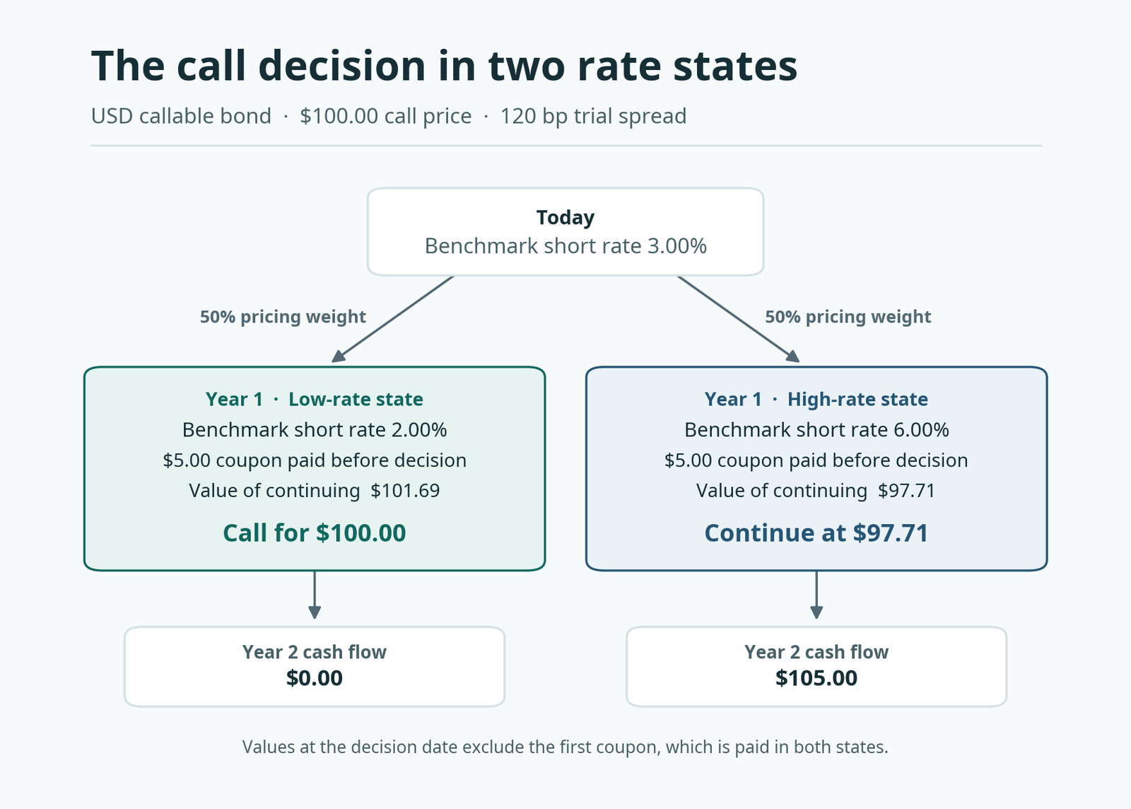
The diagram shows both exercise decisions. The $5.00 first coupon is paid in either branch. When the high-rate branch continues, $97.70574 is the value at year one of the later payment. Actual year-one cash in that branch is $5.00.
Let \(c\) be the $5.00 year-one coupon, \(r_0\) the initial 3.00% benchmark rate, \(V_L\) and \(V_H\) the two after-coupon values, and \(P(s)\) the model’s full price in USD at time zero. Add the first coupon to the weighted value at year one and discount it one period.
\[ P(s)=e^{-(r_0+s)}\left(c+\tfrac{1}{2}V_L(s)+\tfrac{1}{2}V_H(s)\right) \]
At 120 bp the expression inside the parentheses is about $103.85287. Multiply it by \(e^{-0.042}\) to get the unrounded price target, approximately $99.581380615. Use the full precision of that target to recover the spread. At a trial 100 bp, the price is about $99.87471. At 140 bp, it is about $99.28901. The solver raises the spread when its calculated value is above the target and lowers it when the value is below. The fitted OAS here is 120.00 bp.
Reprice the promised schedule on the same benchmark
To compare with the Z-spread, derive the benchmark zero curve from the same tree with no spread added. \(D_1\) and \(D_2\) are the time-zero benchmark discount factors for $1.00 at the end of years one and two.
\[ D_1=e^{-0.03}\approx0.970445534,\qquad D_2=e^{-0.03}\left(\tfrac{1}{2}e^{-0.02}+\tfrac{1}{2}e^{-0.06}\right)\approx0.932580305 \]
The \(t\)-year continuous spot rate is \(-\ln(D_t)/t\), where \(\ln\) is the natural logarithm and \(D_t\) is the benchmark discount factor for that maturity. These factors imply 3.00% and about 3.49000%. For an annual continuous spot rate, adding a constant spread \(z\) multiplies the \(t\)-year discount factor by \(e^{-tz}\), with \(t\) the time in years. Apply that to the promised $5.00 and $105.00 cash flows, holding them fixed for the Z-spread fit. Here \(P_{\mathrm{target}}\) is the same full price in USD.
\[ P_{\mathrm{target}}=\$5.00\, D_1 e^{-z}+\$105.00\, D_2 e^{-2z} \]
At 120 bp, the promised-flow model is worth about $100.39316, which is $0.81177 above the callable price at that spread. A promised-flow fit needs a larger spread to reach the same $99.581380615… target. At about 161.59 bp, the two discounted payments are $4.77445 and $94.80693, calculated with the unrounded fitted spread. Their sum matches the price. The difference between the fitted spreads is approximately 41.59 bp. It comes from the modelled call and should stay paired with that benchmark and model.
Worked example 2. Raise the call price and fit again
Keep the curve, payment schedule, weights and observed full price fixed. The hypothetical contract now allows a call at $101.00 after the first coupon. At the old 120 bp spread, the low-state continuation value is still $101.69319, so the issuer calls at $101.00. The high-rate state still continues. The model price rises to about $100.06082. The option now lets the issuer repay early only at a higher price.
| Call term | Price at the old 120 bp (USD) | Fitted OAS at the same market price |
|---|---|---|
| $100.00 call price | $99.58138 | 120.00 bp |
| $101.00 call price | $100.06082 | 152.72 bp |
Refit by trying higher spreads until the price returns to the original unrounded target. At about 152.72 bp, the low-state continuation value is $101.36096 and the high-state continuation value is $97.38654. The low state is still called and the high state still continues. The new spread is 32.72 bp higher because the investor receives more in the call state at the old spread. For a real bond, a different call term could also change the market price. Holding it fixed here isolates the change in the model fit.
Practice questions
Choose one answer per question. Use the stated assumptions and round final results only. Any dollar amounts are in USD.
1. Make the call decision
Just after a coupon, continuation is worth $102.00 in one state. The issuer may call for $100.00 and chooses the lower-cost action. What value should the model give the investor at that node?
2. Place the first coupon
A $5.00 coupon has just been paid when a model computes a $100.00 call value and a $96.00 continuation value in equally weighted states. Before discounting year one back to today, what amount combines that coupon with the state values?
3. Fit the market price
At a trial spread the option-aware model is above the observed full price. With a decreasing price function as in the chapter, which adjustment moves it toward the price?
4. Read the state weights
The teaching tree assigns equal risk-neutral weights to two year-one states. What does that tell you?
5. Read the comparison with Z-spread
In the model, a $100.00 call gives 120.00 bp OAS and 161.59 bp promised-flow Z-spread at the same price on the same benchmark. Which reading fits the example?
6. Change the call price
You increase the strike from $100.00 to $101.00 with all other inputs as in the lesson. At the old spread, the call still binds in the low state and the high state continues. What happens at the old spread?