The Security Market Line and How to Read It
In this chapter
Intermediate
The security market line (SML) graphs the expected return implied by CAPM for each level of market beta. Put beta on the horizontal axis and expected return on the vertical axis. A forecast above the line exceeds the model’s required return at that beta. A forecast below it falls short of that model estimate.
Plot the intercept and read the slope
Use the same model inputs for every point on the line. In this example the inputs are hypothetical one-year nominal USD simple total returns, including income, before fees and taxes. The risk-free return is 3.00% and the expected market risk premium is 6.00 percentage points (pp). Assume the standard CAPM setup, with beta measured against the same market whose premium you use.
\[ \mu_{\mathrm{SML}}(\beta)=r_f+\beta\,\mathrm{MRP}. \]
\(\mu_{\mathrm{SML}}(\beta)\) is the model-implied expected return at beta \(\beta\), \(r_f\) is the matching risk-free rate, and \(\mathrm{MRP}\) is the expected market premium over that rate. Beta is unitless. In the example, the slope is six percentage points of expected return per additional unit of beta. The vertical intercept is 3.00%, because a beta of zero adds zero premium. At a beta of one the line gives 9.00%, the expected return on the market itself.
Worked case. Plot model points and compare a forecast with the line
| Beta (unitless) | CAPM-implied one-year return | Interpretation |
|---|---|---|
| 0.00 | 3.00% | Intercept at the risk-free rate |
| 0.80 | 7.80% | Smaller exposure than the market |
| 1.00 | 9.00% | Market reference point |
| 1.20 | 10.20% | Larger exposure than the market |
| 1.50 | 12.00% | One and a half times the market premium above the baseline |
At beta 0.80, multiplying \(0.80(6)=4.80\) gives the premium in points. Add 3.00% and plot \((0.80,7.80\%)\). The same calculation at beta 1.50 gives the point \((1.50,12.00\%)\). All model points lie on the same straight line.
Suppose you expect the 0.80-beta stock to earn 9.00% using your own separate forecast. Plot that at the same horizontal position. Its vertical gap is \(9.00\%-7.80\%=+1.20\) pp. That is a positive forecast gap relative to CAPM. In general, \(g_i=F_i-\mu_{\mathrm{SML}}(\beta_i)\), where \(g_i\) is the gap in percentage points, \(F_i\) is your forecast as a percent, and \(\beta_i\) is the estimated beta of asset \(i\). It could come from a different view of the stock’s cash flows, a questionable risk estimate or a limitation in the model.
Change one input and keep the forecast fixed
Worked case. The beta estimate moves the stock across the line
Suppose a better-aligned data series puts the stock’s beta at 1.20. Keep its forecast at 9.00%, and hold the risk-free rate and market premium fixed. The stock’s forecast point moves right along the 9.00% level. The line itself stays where it is.
At beta 1.20, the CAPM return is \(3.00\%+1.20(6.00\%)=10.20\%\). The new gap is −1.20 pp. The same forecast moved from above to below the line because the model now assigns more market exposure to the stock. At beta 1.00 the forecast exactly meets the line. If the best evidence leaves beta somewhere between 0.80 and 1.20, your conclusion about the sign of the gap depends on where within that range the estimate lands. A gap is only as credible as the forecast and the model inputs used to calculate it. A one-year realised return above the line also does not establish a reliable forecasting advantage.
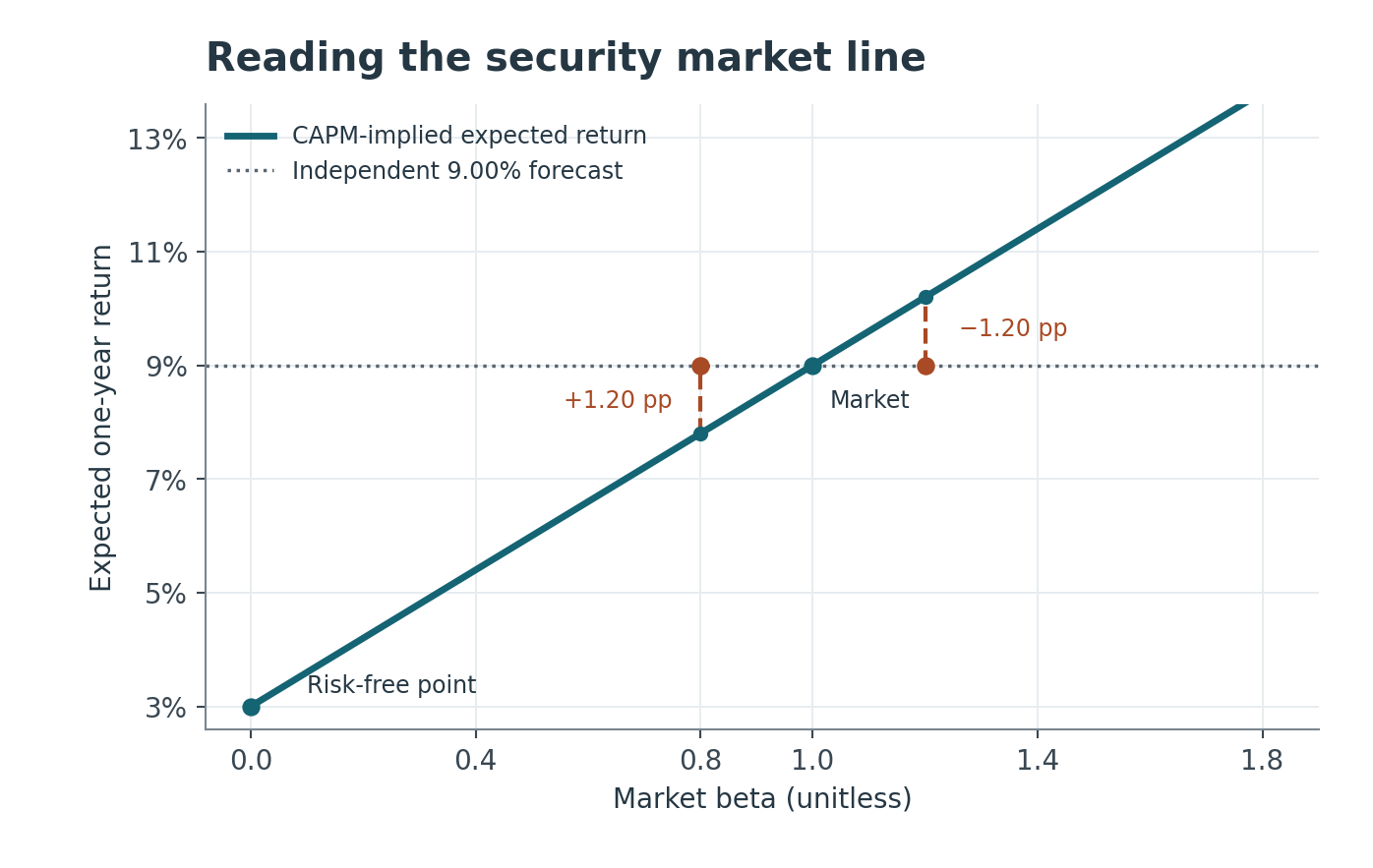
Changing the premium would change the slope of the line. With the risk-free rate fixed, every line still crosses at the same intercept. Changing only one asset’s beta instead moves where you look along an unchanged line.
Check which risk measure belongs on each graph
| Graph | Horizontal axis | What each point represents |
|---|---|---|
| Security market line | Market beta | CAPM’s expected return for a security or portfolio at that market sensitivity |
| Capital allocation line | Total return standard deviation | A mix of one specified risky portfolio and the risk-free asset |
At beta zero on the SML, a security can still have sizable volatility from sources outside the market exposure. At zero volatility on the capital allocation line, the mix is entirely in the risk-free asset in the basic setup. The risk-free rate chapter explains the importance of matching the rate to the payoff horizon in either calculation.
Practice questions
Choose one answer per question. Round only the final result where needed.
1. Read the intercept
The security market line uses a risk-free rate of 2% and a market premium of 5 pp. What is its vertical intercept?
2. Find the market point
The line has an intercept of 3% and a slope of 4 pp per unit of beta. What are the market point’s coordinates?
3. Calculate a forecast gap
At beta 1.50, the risk-free rate is 2% and the premium is 4 pp. Your separate return forecast is 7%. Where does it sit?
4. Change the market premium
The expected market premium rises from 4 to 6 pp and the risk-free rate is fixed. What changes on the graph?
5. Choose the right horizontal axis
Which pair identifies the horizontal axes of the SML and the CAL?
6. Read a model-relative forecast
An asset’s independent forecast is above the SML. What is established?