Beta and How to Measure Market Sensitivity
In this chapter
Intermediate
Beta measures how sensitive a holding’s return is to changes in a chosen market return. A beta of 1.5 means that a one-percentage-point difference in the market return is associated with a 1.5-point difference in the holding’s fitted return. The holding can still move by a different amount in any particular period.
Match the return dates before fitting a slope
Pick a market proxy that represents the exposure you want to measure. Align both series over the same intervals, using the same currency and kind of return. In these examples the data are hypothetical nominal USD monthly simple total returns including income and before fees and taxes. The broad equity proxy and both holdings share the same four dates. We fit a line with an intercept. Four months keep the calculation visible.
\[ \hat\beta_i=\frac{s_{im}}{s_m^2}. \]
\(\hat\beta_i\) is the estimated slope for holding \(i\), \(s_{im}\) is its sample covariance with market proxy \(m\), and \(s_m^2\) is the sample variance of that proxy over the same paired dates. Covariance and variance have the same return units squared, leaving beta unitless. Both divide their sums by \(n-1\), where \(n\) is the number of paired observations. Those denominators cancel in the ratio. You can think of the fitted return as the holding’s average plus beta times the market’s departure from its own average. The market average gives you the starting point for the comparison. If the market series is constant, its variance is zero and you cannot estimate the slope from it.
Historical beta for CAPM is often estimated using asset and market returns above the matching risk-free return. Subtracting the same constant risk-free return every month simply moves both sample means by that constant, so the slope below also fits that case. If the risk-free return varies month to month, rebuild the two aligned excess-return series first.
Worked case. Estimate beta from four matched months
| Month | Market return | Fund X return | Market deviation (pp) | X deviation (pp) | Product (pp²) |
|---|---|---|---|---|---|
| Jan | −6% | −8% | −6 | −9 | 54 |
| Feb | −2% | −2% | −2 | −3 | 6 |
| Mar | +2% | +4% | +2 | +3 | 6 |
| Apr | +6% | +10% | +6 | +9 | 54 |
| Sum | 0 | 0 | 120 |
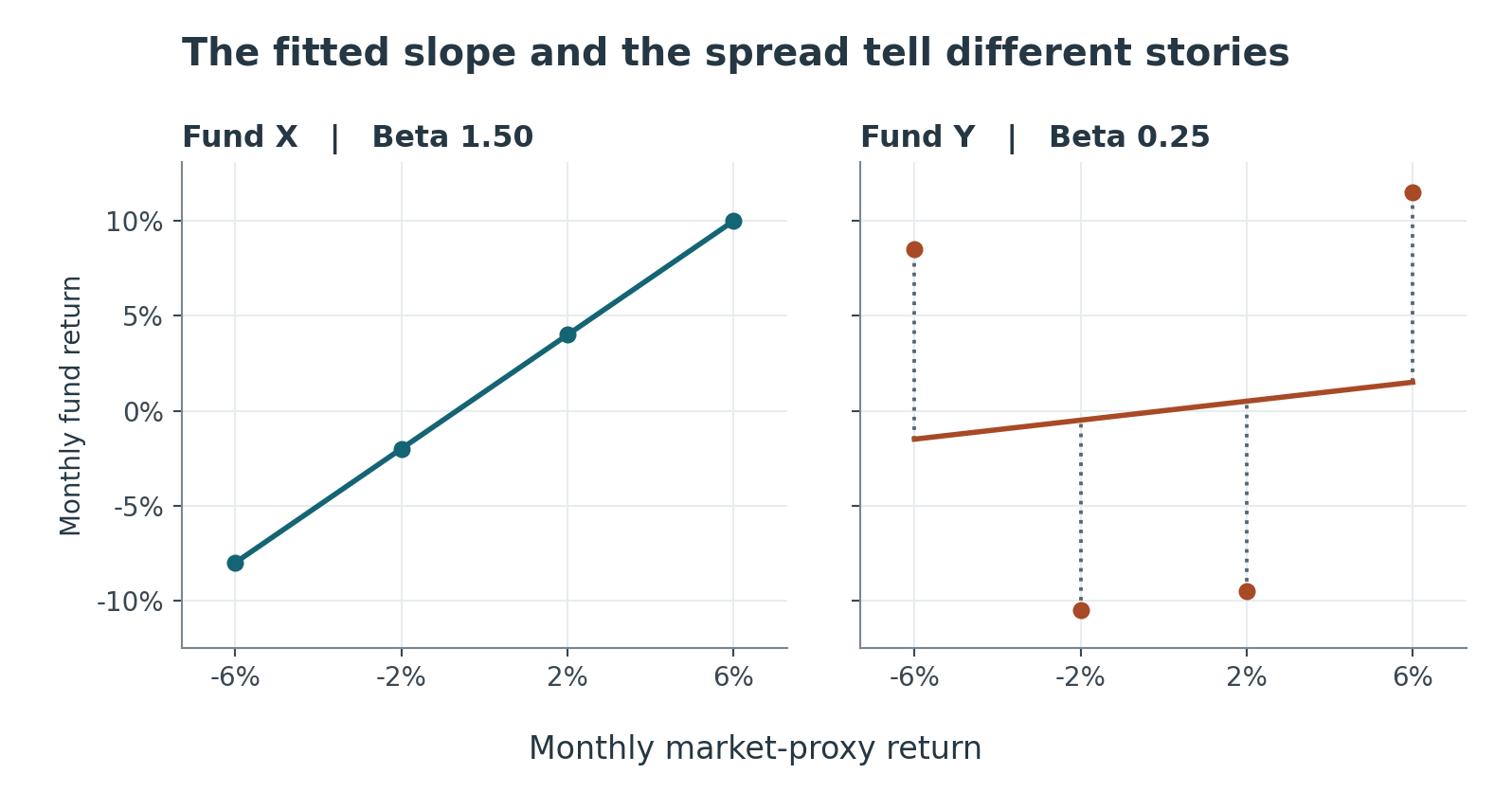
The market mean is 0% and X’s mean is 1%. The squared market deviations sum to \(36+4+4+36=80\) pp². Beta is \((120/3)/(80/3)=\mathbf{1.50}\). The fitted line goes through the mean pair. When the market is two points below its average, the fit puts X three points below its own 1% average. That gives a fitted X return of −2% in that month. The formula allows negative or greater-than-one slopes.
Look at what the market slope leaves unexplained
Worked case. High volatility can come with low beta
Keep the same market series. Fund Y’s mean is 0%. Here are Y’s four returns, the market-linked fit and the difference from the fit, called the residual.
| Month | Market return | Fund Y return | Fitted Y return | Y residual (pp) |
|---|---|---|---|---|
| Jan | −6% | +8.50% | −1.50% | +10.00 |
| Feb | −2% | −10.50% | −0.50% | −10.00 |
| Mar | +2% | −9.50% | +0.50% | −10.00 |
| Apr | +6% | +11.50% | +1.50% | +10.00 |
The paired products around the means are −51, +21, −19 and +69 pp², a sum of +20. Beta is \(20/80=\mathbf{0.25}\). With both means zero, the fitted return is one-quarter of the market return. Y’s own squared deviations sum to 405 pp², so its sample volatility is \(\sqrt{405/3}=\mathbf{11.62}\) pp. X’s corresponding volatility is \(\sqrt{180/3}=\mathbf{7.75}\) pp. Y moves around more in total, while its paired moves line up less with the market.
In this example the residuals contribute 400 of the 405 squared points in Y’s total sum, with the fitted market movement contributing the other five. That split holds here because the residuals from the fitted line are uncorrelated with the market in the sample. A low beta leaves room for issuer-specific shocks or exposure to drivers the chosen index misses.
Check how the estimate changes with a reasonable proxy, return frequency or window. Make sure the benchmark moved enough to support a slope. Very little market variation can make the estimate sensitive to a few unusual asset returns. Review the paired plot for a single period that pulls the line around. Different holdings or business conditions can change the relationship. The slope is an estimate for the paired data and cannot tell you the next return with certainty.
Practice questions
Choose one answer per question. Round only the final result where needed.
1. Calculate a slope
The covariance of a holding with a market proxy is 30 pp², and the market variance is 20 pp². What’s beta?
2. Interpret the fitted response
Beta is 0.60. For a three-percentage-point lower market return, what change does the fitted line give in the asset’s return?
3. Handle a flat proxy
The market proxy has the same return every month. What’s the beta against it from these observations?
4. Read high volatility and low beta
An asset has high volatility and beta of 0.20. Which interpretation fits?
5. Read a negative slope
Market variance is positive and covariance with a holding is negative. What is beta’s sign?
6. Compare two proxy estimates
You use the same asset history with a broad domestic index and a sector index and get different betas. What should you check first?